The Harmonic Series Strikes Again

February 28, 2020

published May 17, 2025

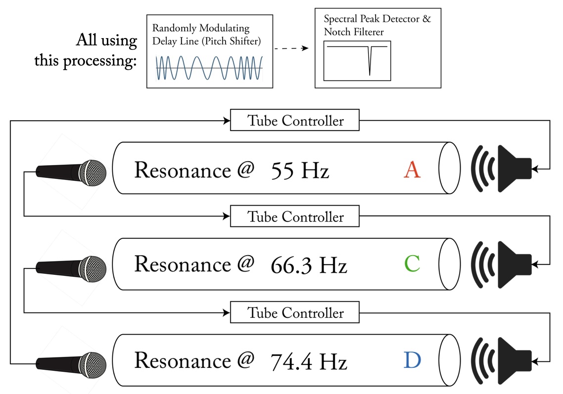
My composition hollow, includes large PVC tubes that are used in a complex audio feedback system. The three tubes (all four inches in diameter) are cut to lengths of 10 feet, 8.4 feet, and 7.5 feet in order to achieve resonances at 55.8 Hz (~A1), 66.3 Hz (~C2), and 74.4 Hz (~D2) respectively.

A recording of a performance of hollow was used as the tape part in the fifth movement of arco. Each of the three tubes were recorded separately enabling the various lissajous plots and “similarity” matrices seen in the video of that movement by comparing different pairs of tubes: (A and C) (C and D) (A and D).

Each can be controlled through digital processes to direct the system’s resonance toward particular frequencies or, alternatively, allowed to behave autonomously, being regulated by negative feedback mechanisms in the feedback signal path. In each case, the tubes act as filters, creating resonance at frequencies in a harmonic series, the fundamental of which is based on the length of the tube. As a whole system, the three tubes can be operate in parallel as three different feedback systems, or in series, creating one large feedback system that circulates through all of them.

After initially discovering the beautiful tones that sound when a feedback loop is created in one tube, I then chose to add two more tubes of different lengths to create a richer harmonic palate. Once the three feedback systems were sounding, a clear next experiment was to hear the tubes in series, which, by increasing the complexity of the system, provided some surprising results including a distinct A Mixolydian-ish scale. Continuing to experiment with this instrument and adding feedback saxophone in performance increased the complexity of the system, creating sequences of tones, harmonies, timbres, and gestures that felt very musical. The goal of the following analysis is to understand the emergent properties of this feedback system so that they may be further exploited and/or so that future experiments could build off of this understanding.

Tube Controller

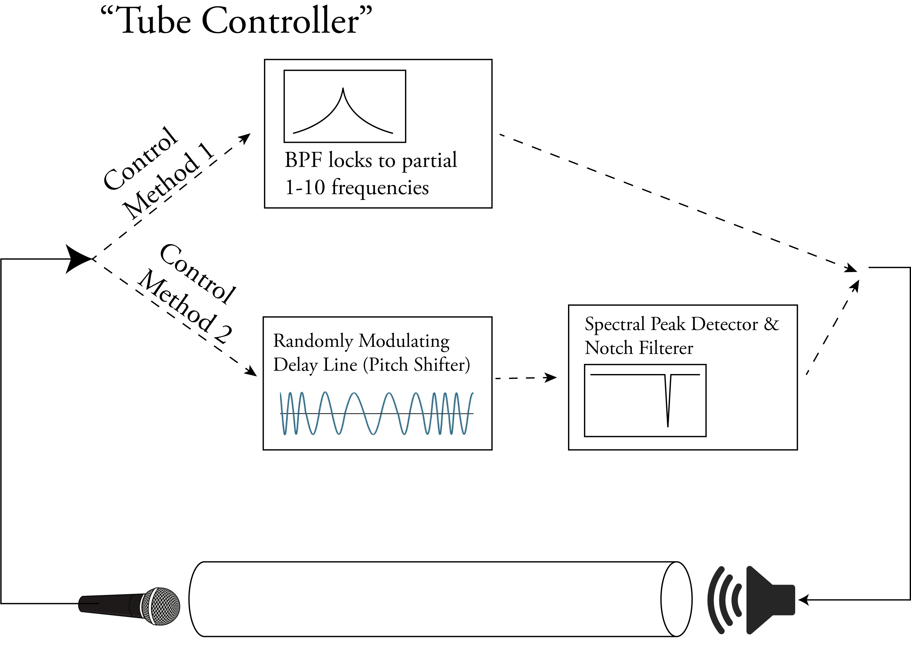
Figure 1: Method for routing and controlling the feedback in the tubes.

Each tube has a microphone at one end and a speaker at the other (both placed directly in front of and facing their respective openings). When the tubes are operating in parallel, the sound that comes out of the speaker travels down the tube, is picked up by the microphone, amplified, and sent back to the speaker, creating a feedback loop. Between the microphone and speaker, this signal goes through SuperCollider to be processed by two compressors, a limiter, a tanh transfer function, and a softclip transfer function to keep the feedback from blowing up and prevent it from clipping or distorting unpleasantly. SuperCollider also enables the performer two ways of manipulating the audio in the feedback path: Partial Mode and Modulation Mode.

Partial Mode

Figure 2: Screenshot of “tube controller” interface for hollow created in the iPad app Lemur. — Figure 2: Screenshot of “tube controller” interface for *hollow* created in the iPad app Lemur.

The first method of manipulation is with a bandpass filter, the center frequency of which is restricted to only be positioned at resonant frequencies of the tube it is controlling (partials 1-10). The performer can freely move the center frequency along a slider that “snaps” to these limited options. The rejection of other frequencies (and resonance of the filter) restricts the feedback from sounding anywhere other than at the partial indicated, however, presence of the tube and multiple transductions involved introduce some analog imprecision into the system, preventing it from resonating at precise integer multiples of its fundamental. Experientially, however, the sound of an overtone series is still very strong. Figure 3 shows a histogram of each tubes' sounding frequencies (while the tubes are operating in parallel). Dotted lines indicate partials for each tube by color. Throughout this analysis the tubes are represented by the following colors:

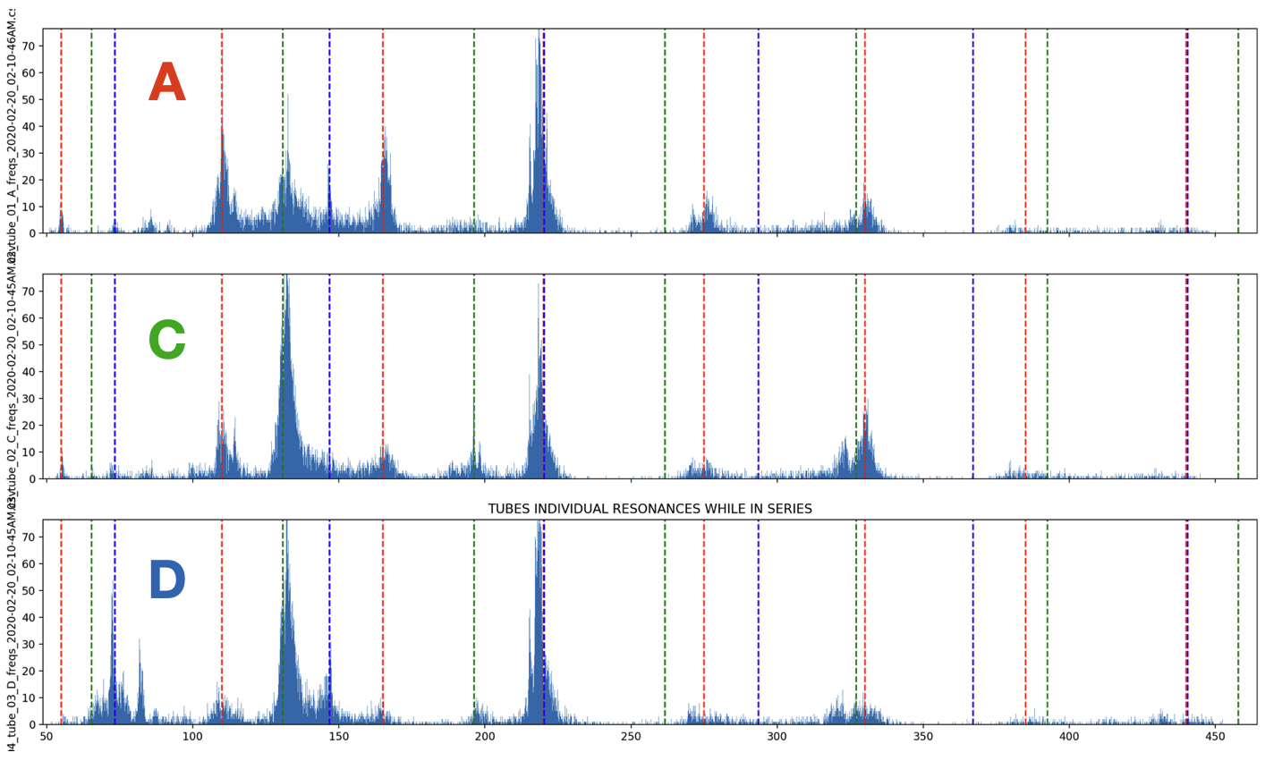
Red: 10 feet (55.8 Hz ~A1)
Green: 8.4 feet (66.3 Hz ~C2)
Blue: 7.5 feet: (74.4 Hz ~D2)

Figure 3: Histograms of tubes’ sounding frequencies when operating independently.

Modulation Mode

The second method of manipulating a tube’s feedback audio is with a combination of a modulating delay line and a feedback suppressor, which allows the tube to behave more autonomously. The modulating delay line (sine wave low-frequency oscillator at 0.01 Hz with a depth of 0.06 seconds) acts as a pitch shifter, “pushing” the signal way from its current resonance. The spectral resonance suppressor uses an FFT analysis (window size = 4096, hop size = 1024) to identify spectral peaks surpassing a given threshold and responds by attenuating the peak with a narrow bell EQ (q = 20) that fades from 0 to -2 dB over 4 seconds. Although -2 dB seems minimal, it continuously adds these bell EQs until the spectral peak is below the threshold. Also, it adds the bell EQ at whatever frequency the phase vocoder is currently reporting for the bin with the maximum magnitude, therefore even if the peak shifts in frequency but stays within the same bin the suppressor will track it. Each bell EQ that is added stays in place for a random length between 14 and 17 seconds. This negative feedback system counteracts the positive feedback of audio amplification, keeping the system from continuously growing in volume, but also preventing it from resting on one resonant frequency for very long.

Performance

Figure 4: Signal flow of tubes in series.

In the opening of hollow, the tubes are in parallel, used in Partial Mode, creating three independent voices used to create three part harmonies with rich beating patterns (Figure 5). After developing these sounds from their lowest to highest register, I begin switching the tubes, one by one, into Modulation Mode allowing the modulated delay line and resonance suppressor to act on the signal, preventing it from remaining at any one partial for long. After letting these overtone series sound for a while, I cross fade to the signal flow that connects the tubes in series (seen in Figure 4), now creating one feedback loop, instead of three. As expected, histograms of the tubes’ analysis frequencies while in series (Figure 4) are more similar to each other showing clear preferences for where, in frequency space, the three-tube feedback system prefers to resonate. The sonic experience of these tubes while in series is a slowly evolving soundscape that draws from tones in an A Mixolydian scale with an added C natural in the lower register (Figure 6). Although only one frequency is most prevalent at any given moment, other pitches from this scale can be heard at various times creating a sense of harmony, especially during moments of transition from one salient frequency to the next.

Figure 5: Plot of tube frequencies for opening of hollow. — Figure 5: Plot of tube frequencies for opening of *hollow*.

Figure 6: Histograms of the tubes’ analysis frequencies while in series.

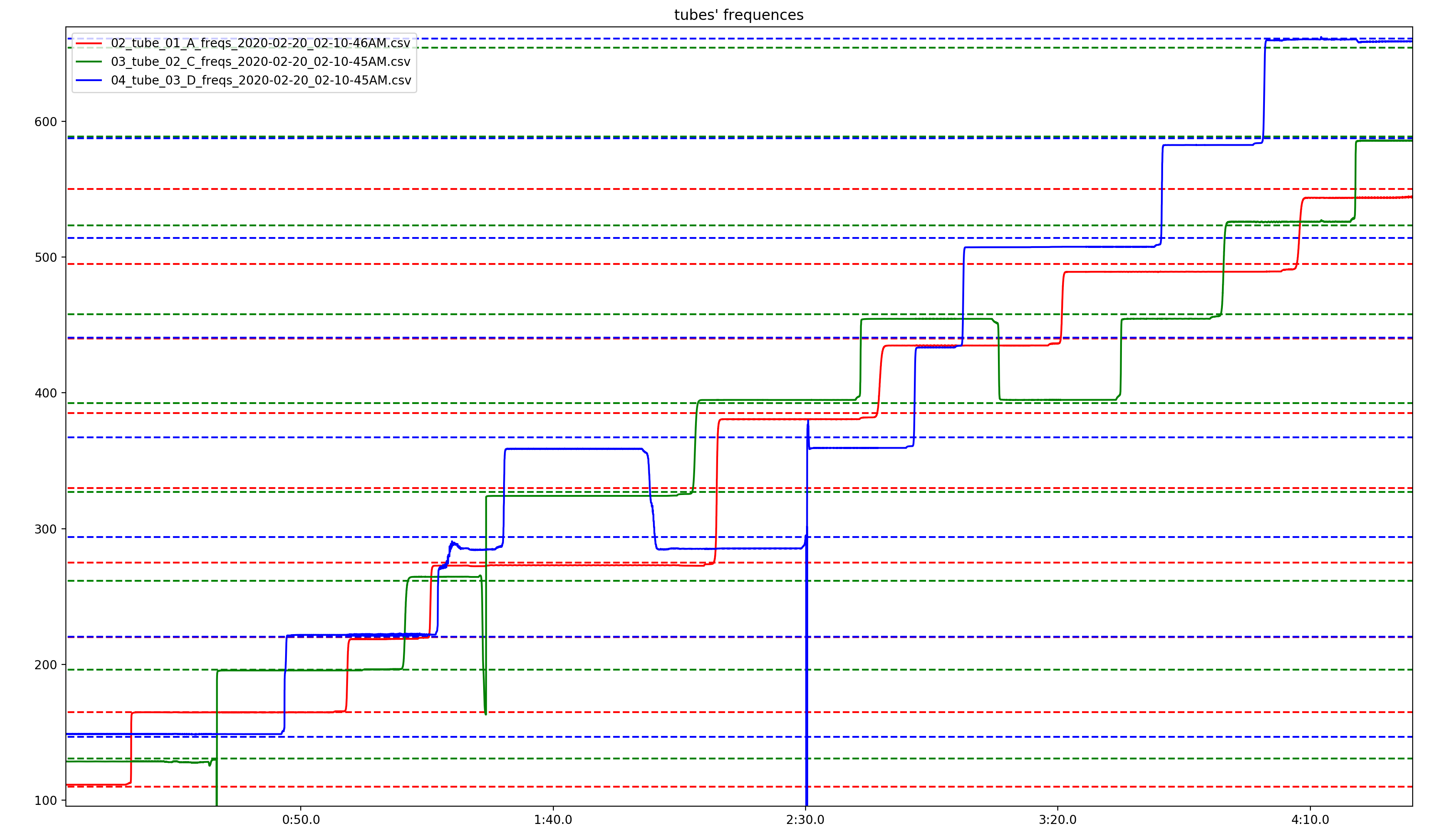
Frequency Cycling

Charting the three tubes’ frequencies though time (as seen in Figure 7) reveals them moving mostly in concert with each other, as well as a clear periodicity in the occurrence of certain frequencies. While this first seems like an indication of emergent behavior resulting from complex interactions, I quickly realized that it is most likely caused by the chosen duration of the bell EQs in the resonance suppressor. The cycle of frequencies seen in Figure 7 is about 20 seconds: just longer than the range of each bell EQ (randomly between 14-17 seconds), accounting for a few seconds for the feedback to build up in a register after the EQs are removed.

Figure 7: All three tubes frequencies though time, showing periodic repetition of certain frequencies.

Tube Interaction

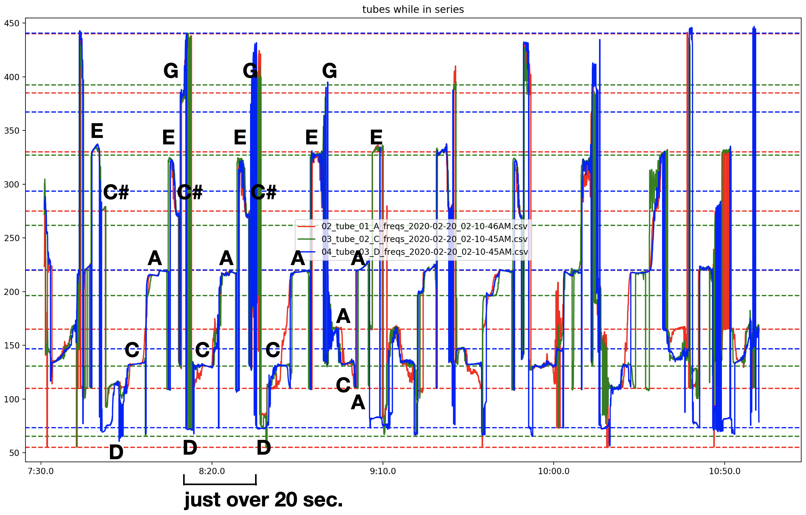
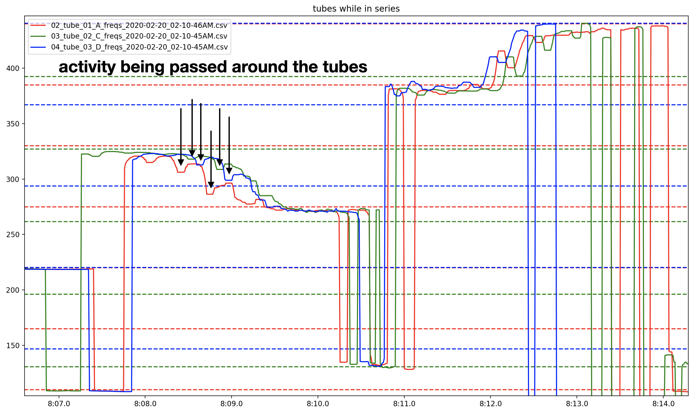
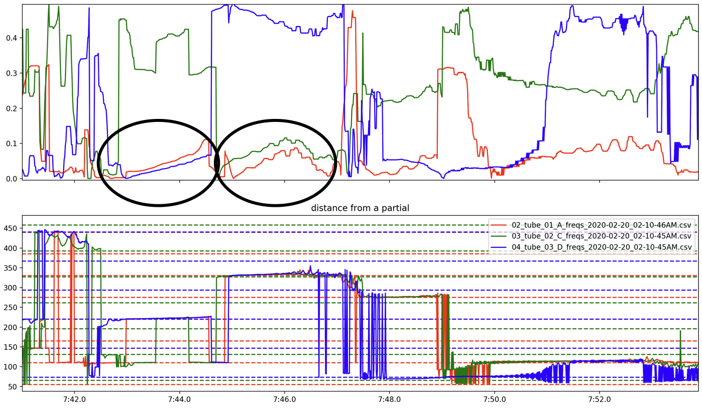
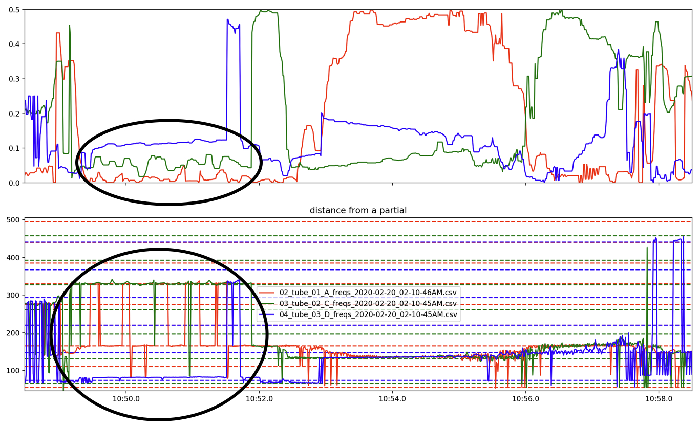
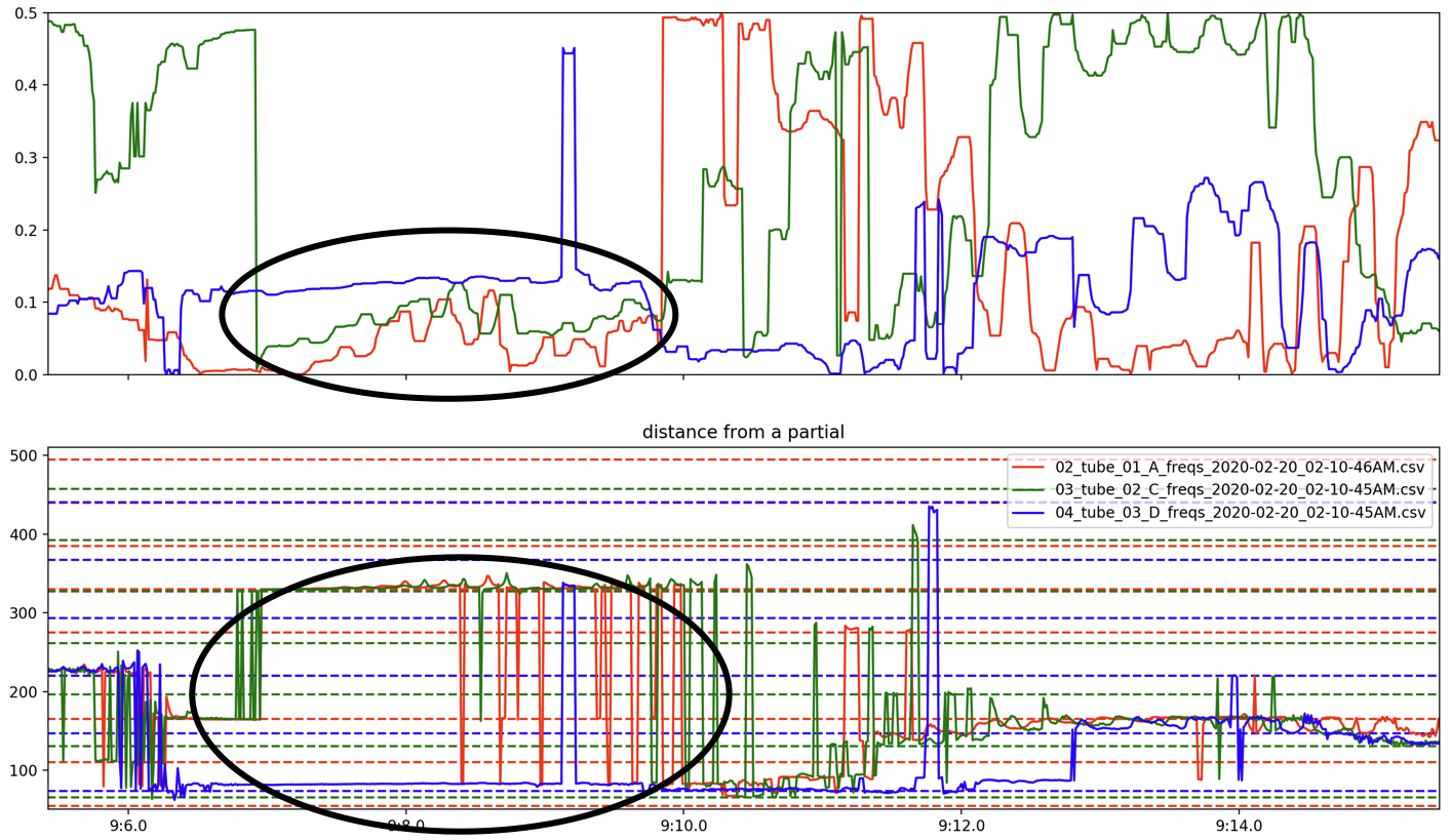
Zooming in on the tubes’ frequency plots displays more complex interactions. Figure 8 shows how a dip in the sounding frequency of the system is passed around the feedback loop through each tube. At 8:08, all three tubes are around 325 Hz, then transition to about 275 Hz by 8:09.6. During this descent, the tubes’ frequencies deviate from each other slightly, revealing a dip in frequency that cycles through tubes: A, then C, then D.

Figure 8: Frequency changes in the three-tube feedback system being passed around the tubes.

The drastic and jittery deviations between partials seen in these graphs can be understood by Figure 9, which plots a sonogram of the tube’s audio recording and overlayed with the pitch tracker line analysis. This shows that the monophonic pitch tracker is responding to other frequencies present in the tube, yet is mostly representative of the tubes’ (and system’s) strongest resonances. Aural perception of the system reinforces the presence of this polyphony.

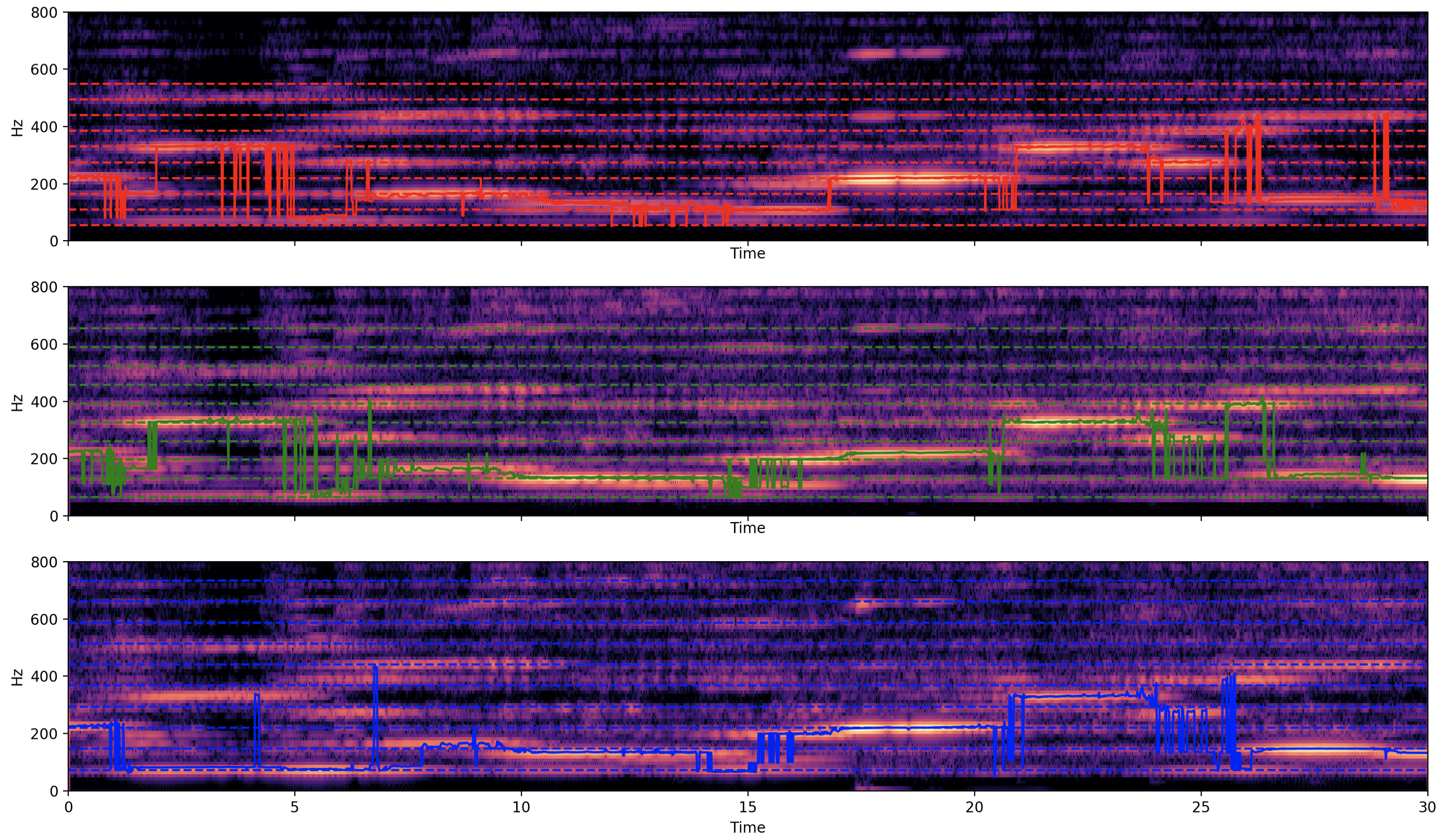
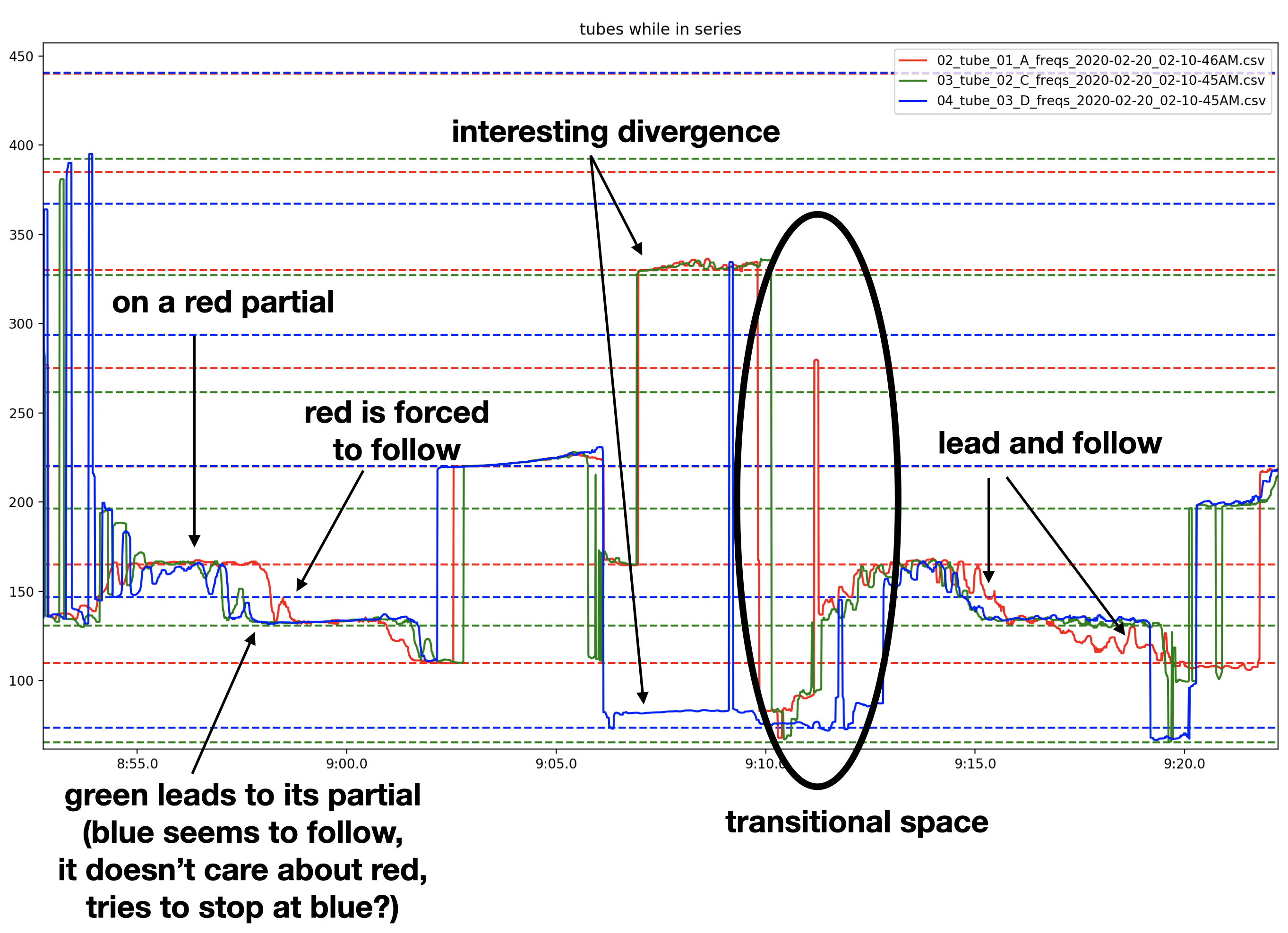
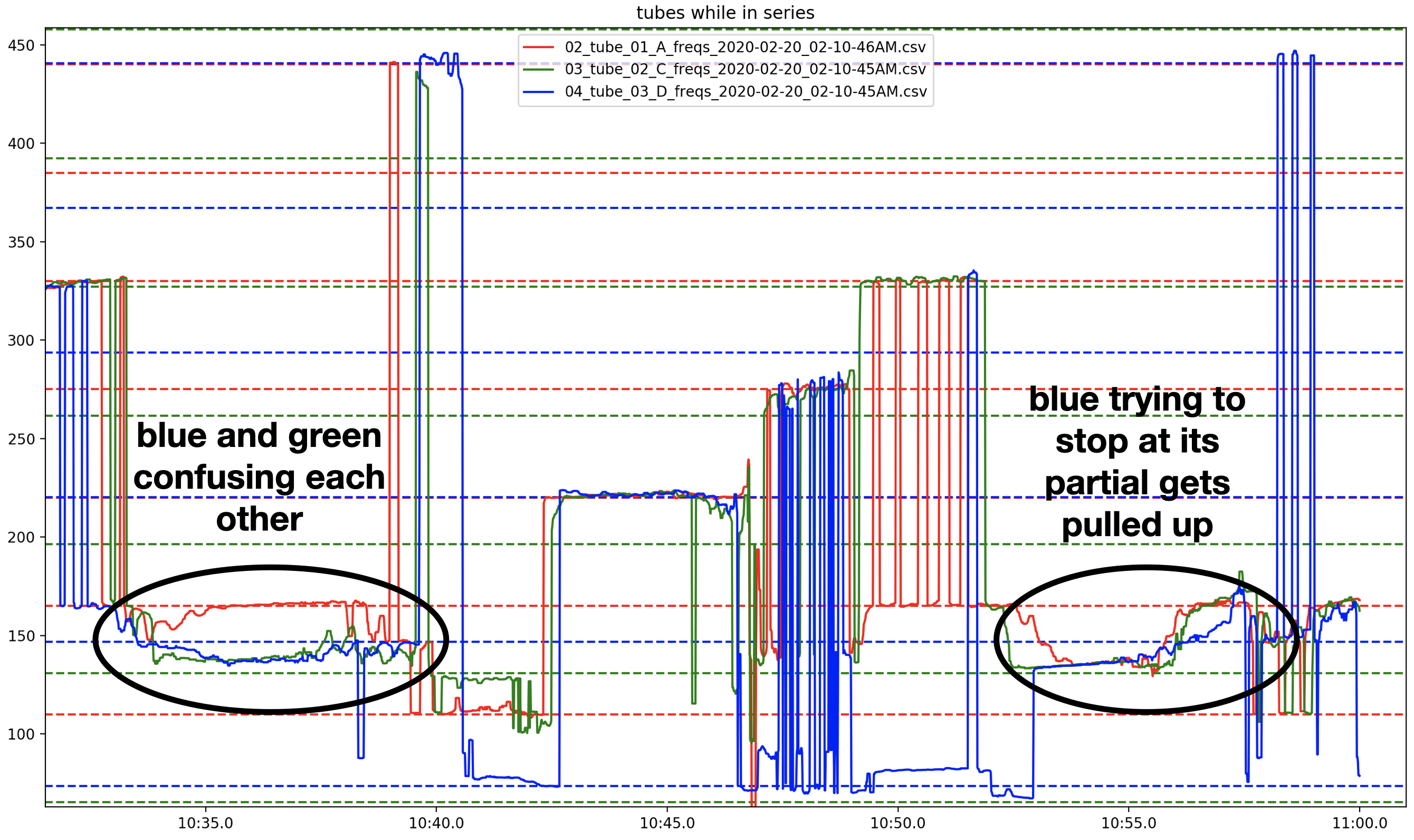
Figure 9: Sonogram of each tube with pitch tracker overlayed.

Figure 10 shows more complex interactions, including (1) how individual tubes can lead the system to one of its own partials, “dragging” the other tubes to join, (2) interesting divergences where one tube will resonate at a frequency very different from the others, and (3) transitional spaces where no clear stability can be observed. Figure 11 shows (1) a moment where the A tube (red) stays steadily on its own partial while the C (green) and D (blue) tubes seem to be “fighting” with each other for which harmonic series to come to rest in and (2) a moment when the system transitions from the second partial of C (green dotted line) to the third partial of A (red dotted line), however, the D tube (blue) seems to resist this motion, attempting to remain at its second partial (blue dotted line) as the system passes by that frequency.

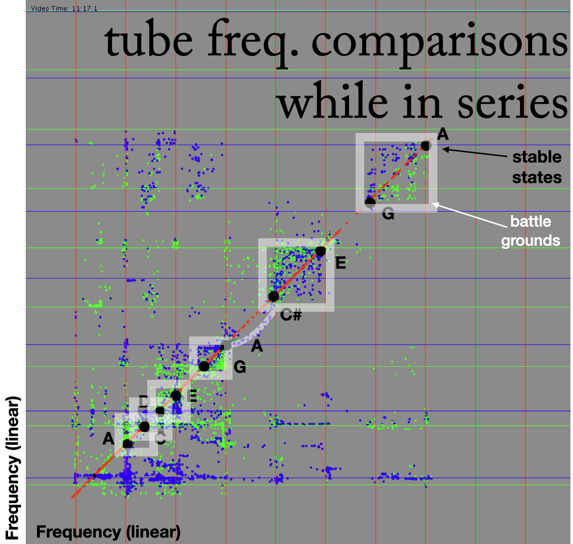
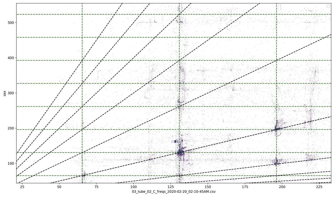
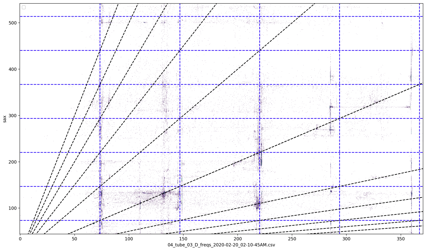
Uncovering Battle Grounds

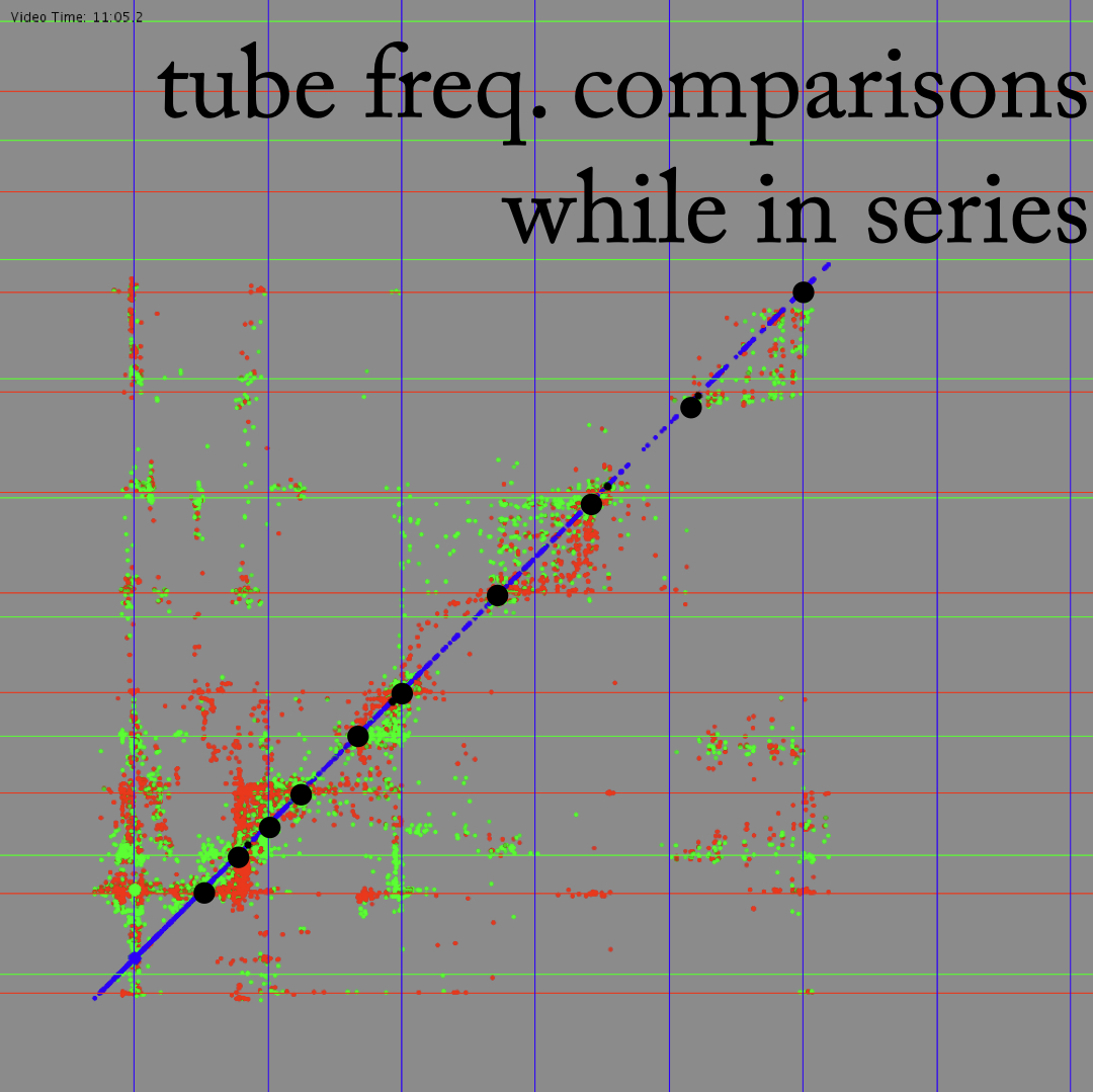
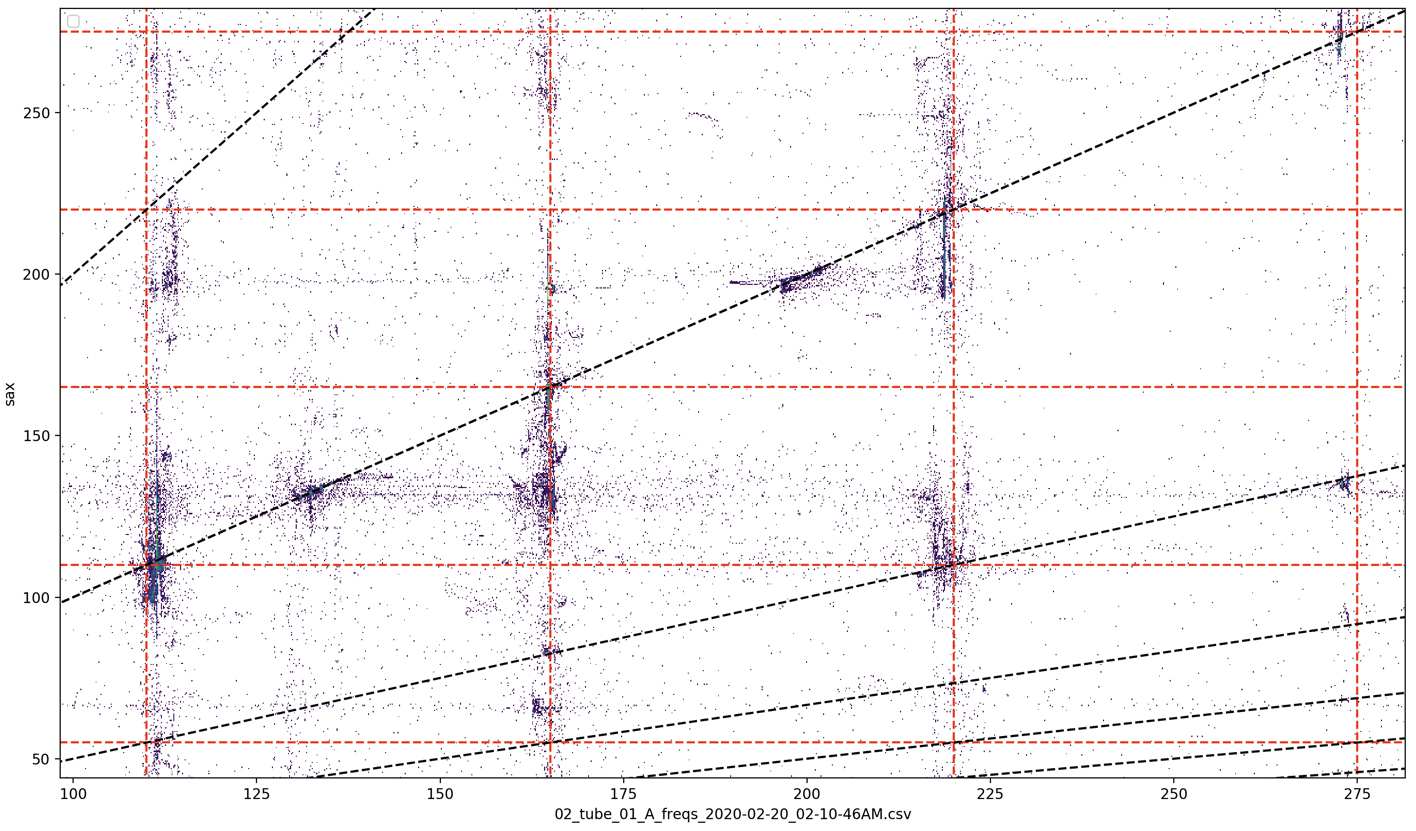
The transitional moments and ensuing “fights” between tubes are the most sonically compelling passages that arise in performance. By further understanding these moments in particular, I hope explore their possibilities and perhaps identify strategies to induce them in other feedback systems. Figures 12, 13, and 14 show two-dimensional histograms of the relation between two tubes’ frequencies while in series. Each point is a moment in time indicating the simultaneous frequency of the two tubes being represented. Bluer points represent more moments in time; a “taller” peak on the histogram. These plots show where in frequency space the two tubes tend to be–more dense clusters represent more time spent in that state. The diagonal line at y=x (or about 45 degrees) represents unisons, where both tubes are at the same frequency. Diagonal lines fanning out from the unison line are integer multiple relations, which would indicate that the tubes are not at the same frequency, but in harmonic relation with each other.

Figure 12: 2D histogram of frequencies in A and C tubes.

Figure 13: 2D histogram of frequencies in C and D tubes. Gray circle represents the stable state seen in Figures

Figure 14: 2D histogram of frequencies in D and A tubes.

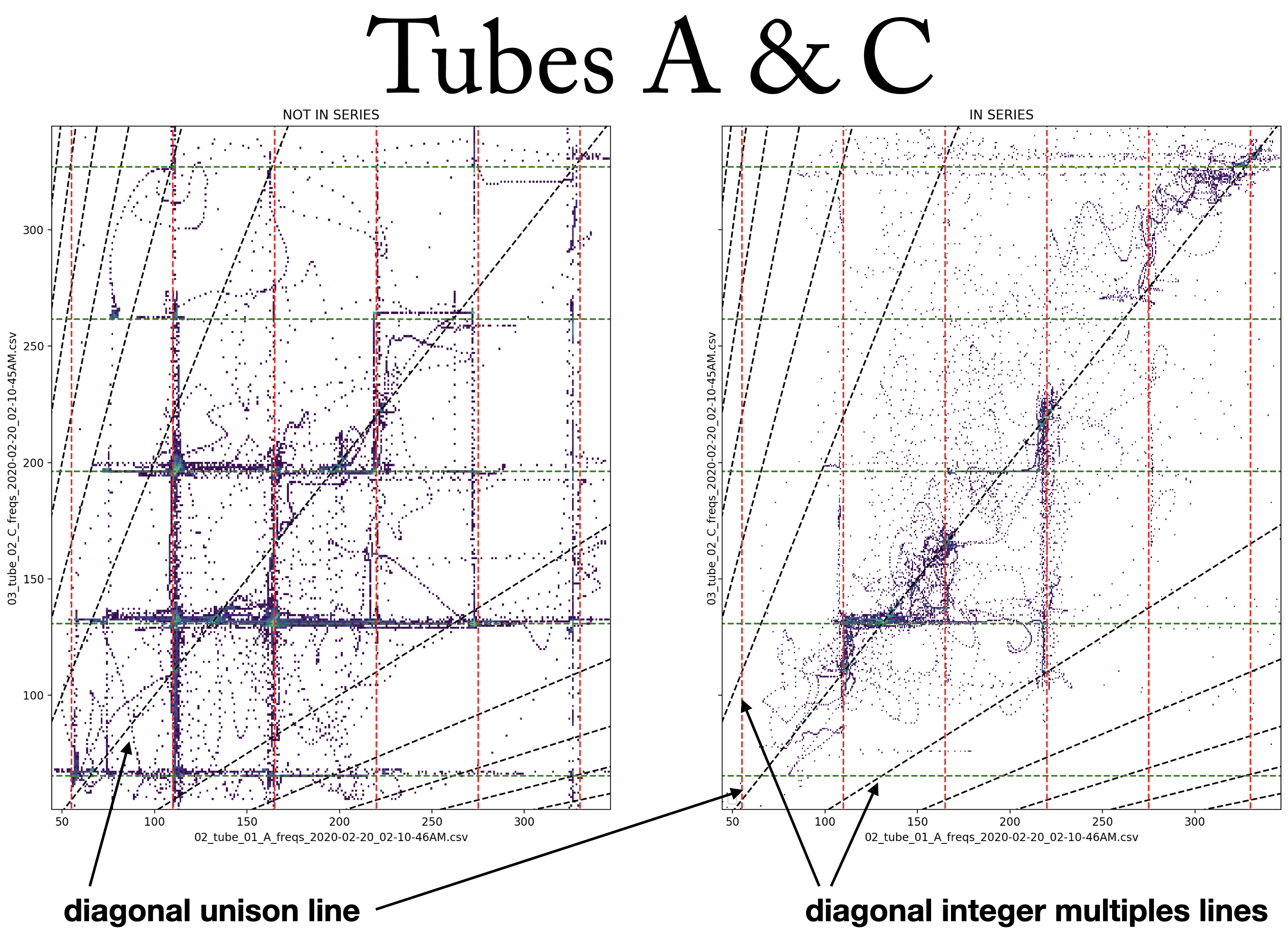
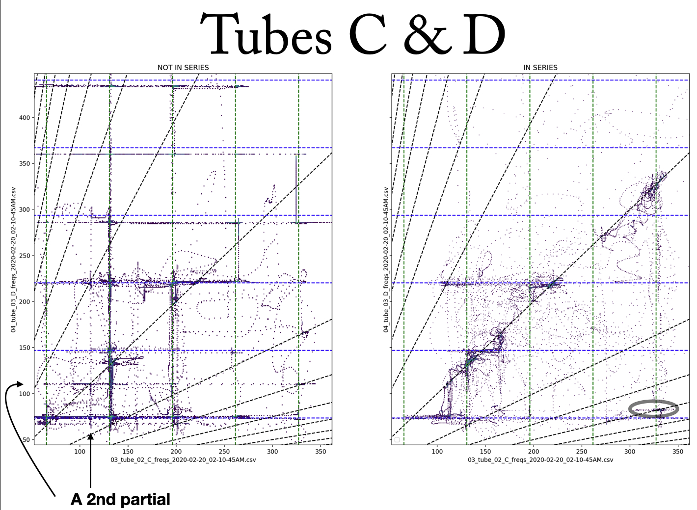
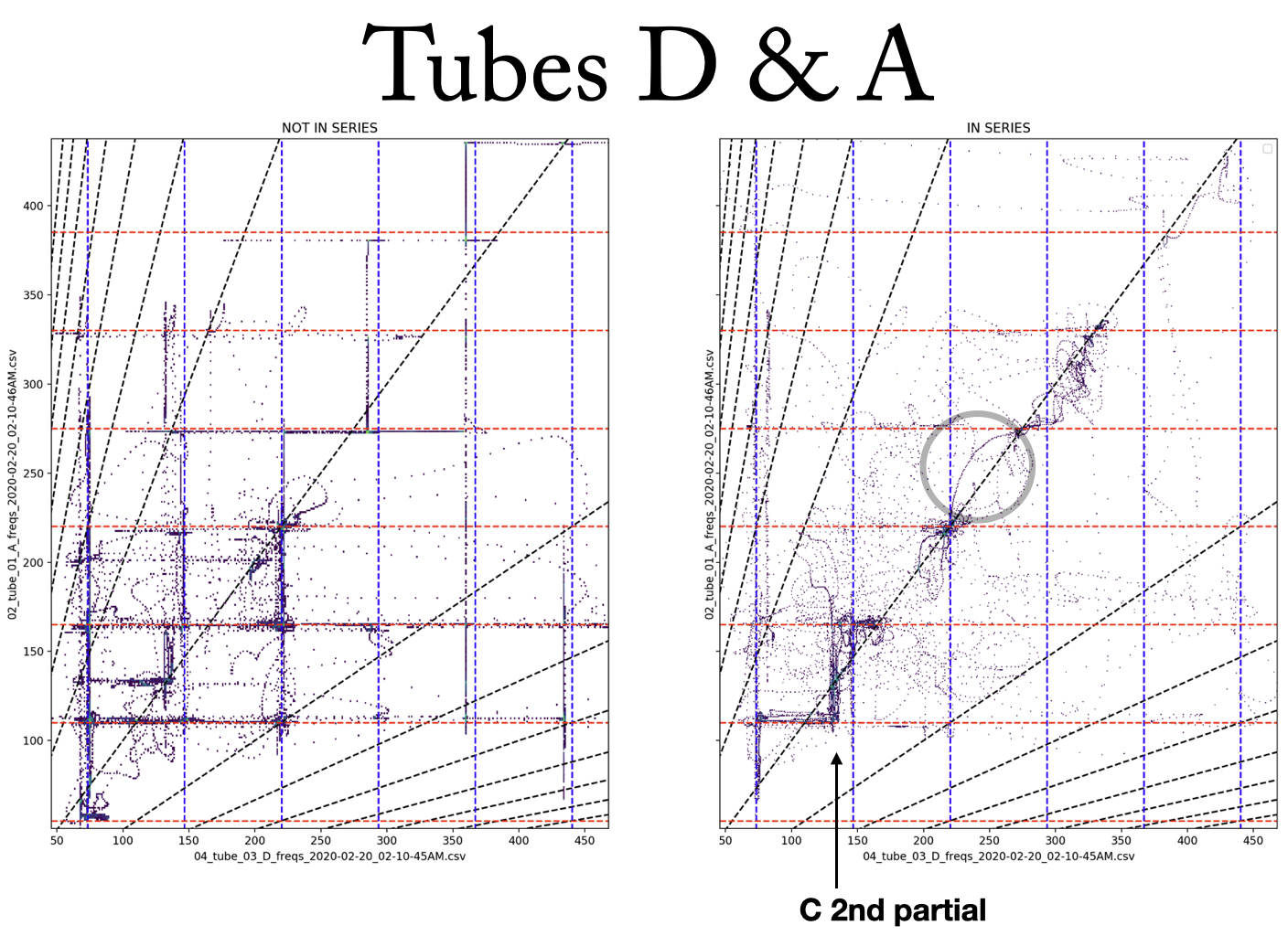
From these plots, one can see that while the tubes are not in series (left side) each tube is independent, mostly sounding its own partials, as expected. While the tubes are in series (right side), however, the points, or “states,” are much more clustered around the unison line, as the system is one feedback loop, sounding (mostly) one resonance. Also, there are clear clusters of states at points along the unison line, indicating locations of stability (stable states, or homeostasis) that the system prefers to resonate at. One can also see looping curves through the space, which can be assumed to be connected into lines through time representing a transition from one stable state to another in which one tube resists leaving its own partial, but eventually is “dragged along” to a stable state not in its harmonic series. For example, the circled arc in Figure 14 shows the system transition from the A tube’s fourth partial (which is roughly also D tube’s third partial), to A tube’s fifth partial, however, the D tube clearly resists this motion initially (the point is trying to maintain its x axis position, therefore the arc starts by moving up instead of diagonal along the unison line). The resonance in the D tube eventually succumbs to the system’s movement, allowing the x position of the point to move to the right, reconnecting with the unison line (the tubes are again in unison) where it intersects the A tube’s fifth partial.

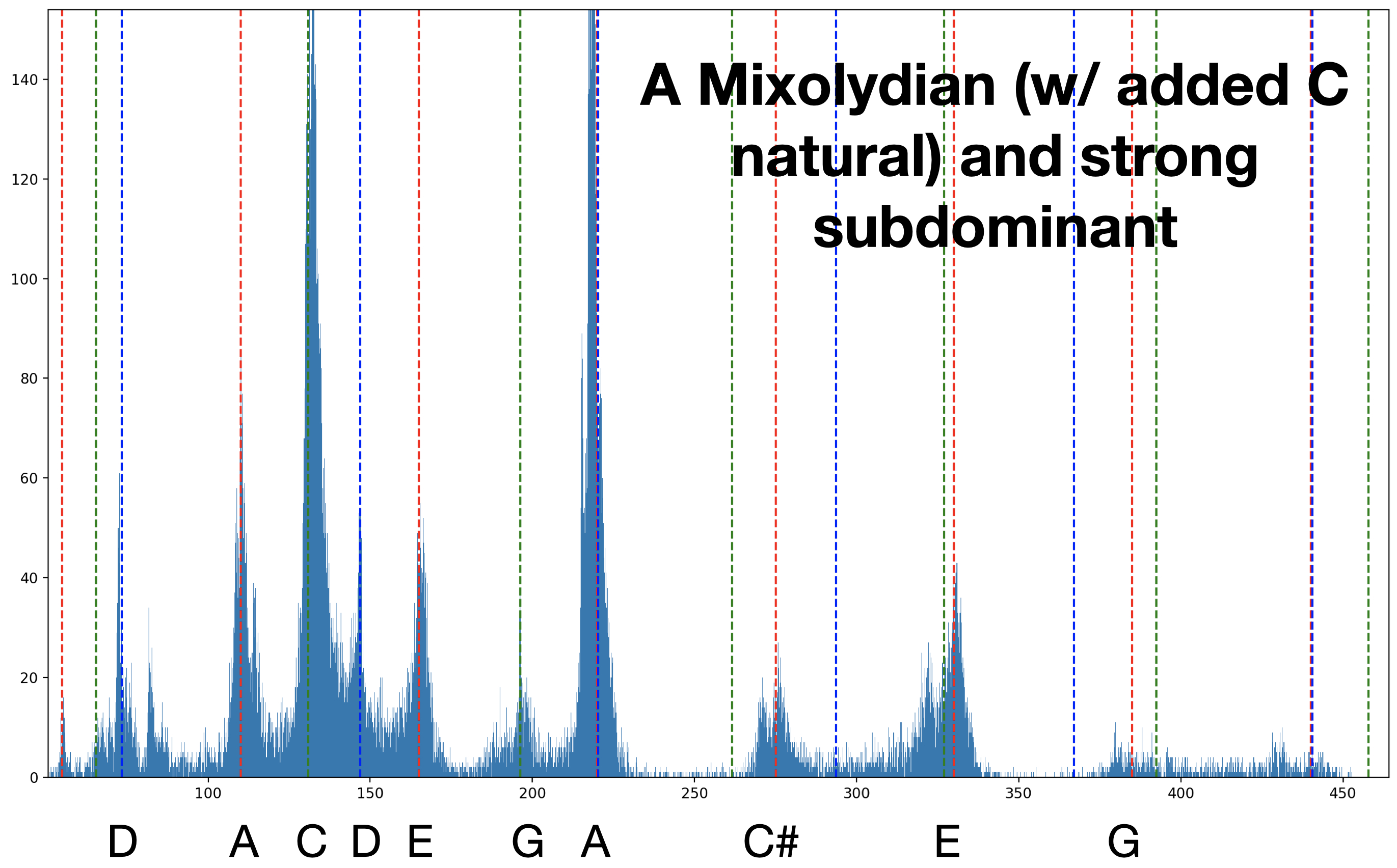
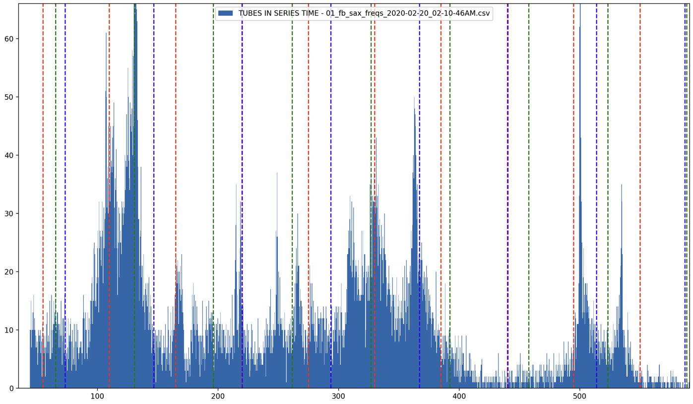
The harmonic content of the listening experience is reflected in the position of stable states, which outline an A Mixolydian scale with an added C natural in the lower register. There is also a strong subdominant presence in the tubes’ performance, created by the D tube. Comparing Figure 3 (histogram of each tube’s sounding frequencies while in parallel) and Figure 15 (histogram of all tubes combined while in series), one sees that the scale of the three-tube feedback system is a combination of some partials from all the tubes. It is important to notice however that although the unison line crosses all possible partials, there are not point clusters at all crossings; there are some partials that the three-tube feedback system does not come to rest at (i.e., resonate at).

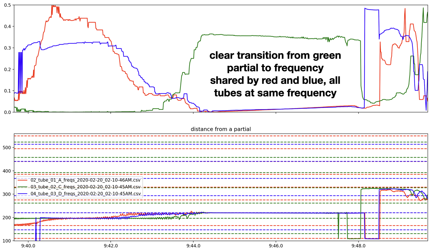
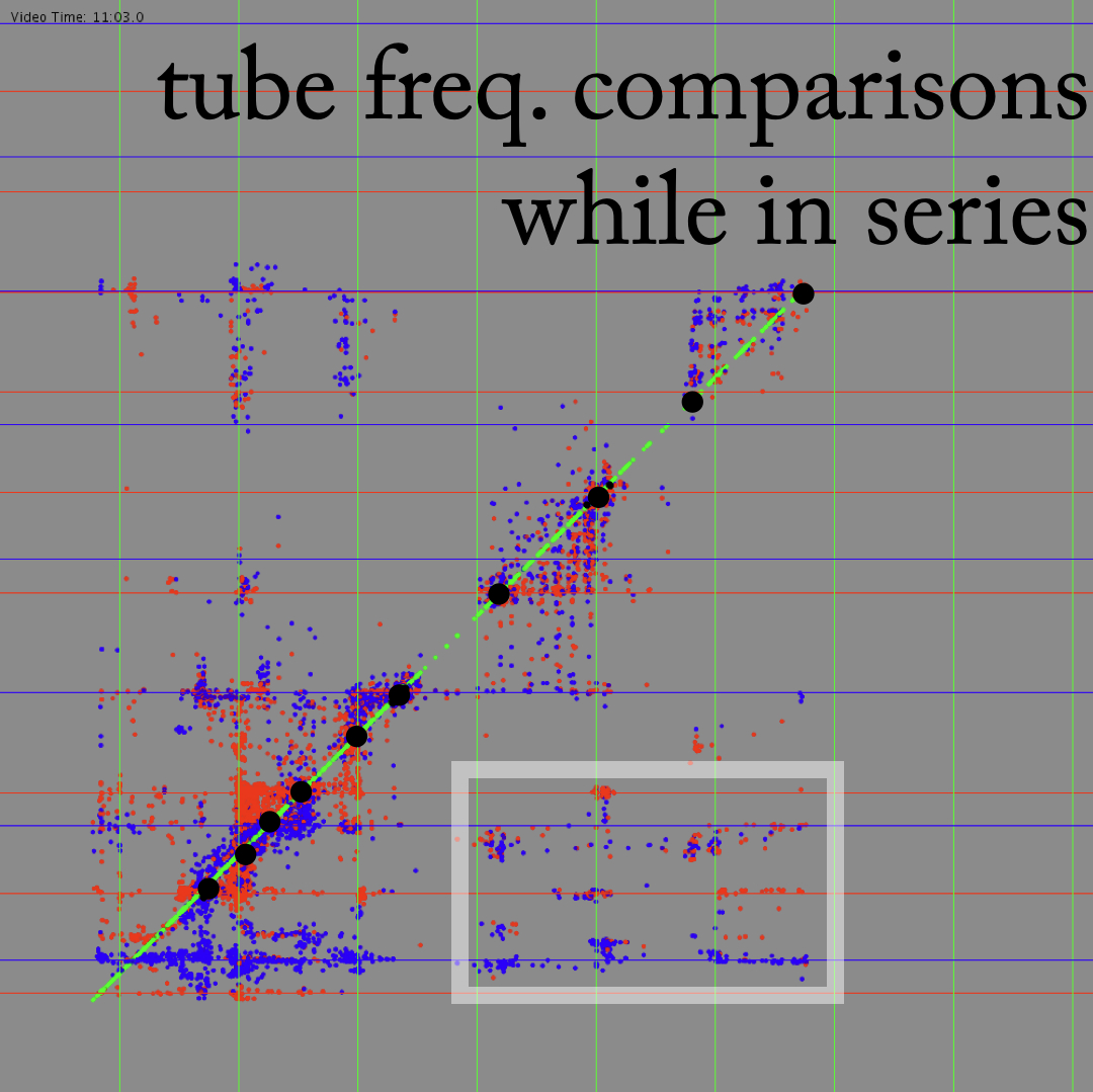
Figure 15: Histogram of all three tubes’ (in series) frequency analyses combined.

In order to analyze how the resonance tendencies of the whole system relate to the different harmonic series of the tubes, Figure 16 shows the normalized distance of each tube’s sounding frequency from its nearest partial (a value of 0.0 distance means it is at a partial in its harmonic series, 0.5 means it is directly in between two of its partials). For any given point in time, this plot shows which tubes are resonating within their harmonic series (close to 0.0) and which tubes are not (close to 0.5). Figure 16 shows a moment that transitions from a stable state only near a C tube partial to a stable state only near partials in the D and A harmonic series. This is easy to see in the bottom graph (the pitch of each tube) as well as the top graph (each tube’s relative proximity to it’s nearest partial). Most stable states are at frequencies that allow two of the tubes to resonate in their harmonic series (there are none that encompass all three); two examples can be seen in Figure 17. While all these examples lie along the unison line, there are some states in the system that seem to be stable, yet are distant from the unison line, for example the same stable state is seen in Figures 18 and 19. The circled area in Figure 13 shows on the two-dimensional histogram the cluster of points very distant from the unison line representing this stable state.

Figure 16: A transitional moment demonstrated by the distance of each tube’s sound frequency from its nearest partial.

Figure 17: Two stable states, each of which is near a partial in two of the harmonic series.

Figure 18: A stable state distant from the unison line.

Figure 19: A stable state distant from the unison line.

The final plotting strategy used to understand this system shows clear “battle grounds” where the tubes are “fighting” over which of the system’s stable states (most of which are in A Mixolydian) to settle on. Figure 20 shows the relation of C tube’s (green dots) and D tube’s (blue dots) frequencies (y axis) in relation to A tube’s frequencies (x axis) (red dots are the relation between A tube and A tube, therefore always on the unison line). The large black dots on the unison line represent the stable states of the system (as seen in Figure 15). One can again see that some partials of tubes are not included as stable states (such as the fourth and fifth partials of D and fourth partial of C). More interestingly, one can see square-shaped clusters of points that use adjacent stable states as the bottom-left and top-right vertices (those on the unison line). Figure 21 shows larger square shapes created by non-adjacent stable states. These squares show a lot of structured activity near these stable states as the system transitions between them. The curved white line seen in Figure 21 (which is the same one in Figure 14 seen from a different angle), again shows the D tube attempting to remain at its third partial on the y axis (pitch A), while the system moves to the C# above it, eventually curving up and also arriving at C#. I refer to these squares as “battle grounds” because they represent the pitch space in which the system is out of homeostasis as the three tubes seemingly “battle” for the system to settle at a state that is within their harmonic series.

Figure 20: Frequency of C and D tubes in relation to A tube and appearance of “battle grounds.”

Figure 21: Zoomed in region of “battle grounds” revealing a larger battle ground created by the non-adjacent stable states C natural and E natural.

The “battle grounds” shown in Figures 20 and 21 can also be seen (without white boxes) in Figures 22 and 23, as well as other seemingly non-arbitrary structural shapes further off the unison line. Video representations of these plots, which more clearly demonstrate the “battles” as they occur through time, can be viewed below.

Figure 22: “Battle grounds” seen by comparing A and C tubes.

Figure 23: “Battle grounds” seen by comparing A and D tubes.

Analysis Excerpts:

Analysis Excerpt 1
Analysis Excerpt 2
Analysis Excerpt 3

Full Analysis:

Feedback Saxophone

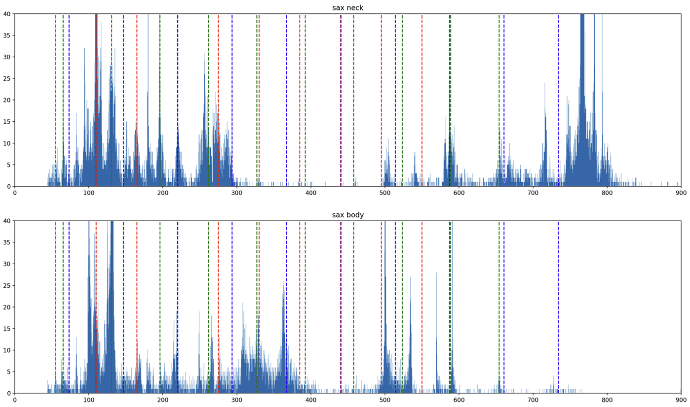
The saxophonist is also performing a feedback loop created by placing a small lapel microphone in the neck of the instrument (the mouthpiece is removed). The sound transduced by this microphone is amplified through the house stereo speakers (not speakers used for the tubes) creating a feedback loop that is responsive to the resonance of the saxophone body. Before performing with the whole saxophone body, the microphone is first placed in only the neck, creating a much smaller tube for resonance. Once the entire saxophone body is attached, the resonating length of tube can be manipulated by the keys, changing the pitch and offering feedback performativity to the saxophonist. Figures 24 and 25 are histograms of the resonance of the saxophone feedback system (as analyzed from the performance audio) which shows more diversity of frequency content than any single tube, but also is clearly influenced by the tubes’ resonances–often sounding frequencies that are in in the tubes’ harmonic series.

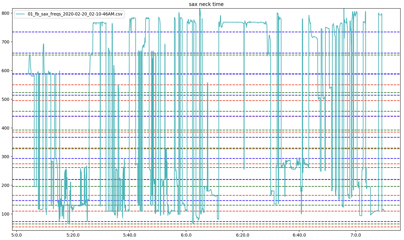
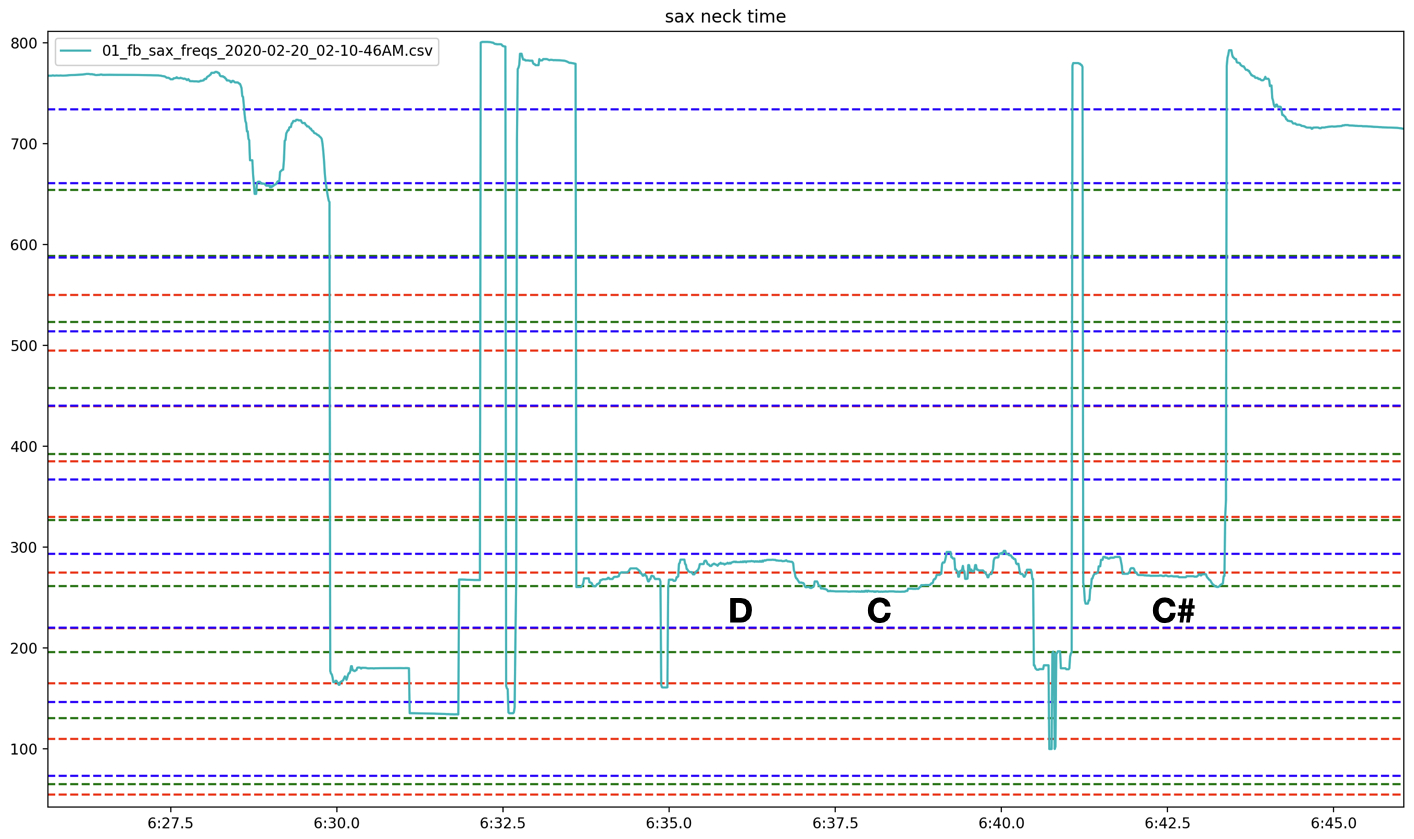
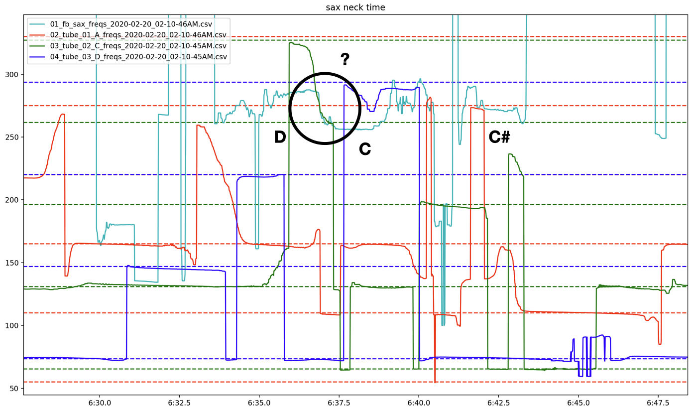
Figure 24: Resonances histograms of saxophone neck (top) and full construction (bottom) as heard in hollow. — Figure 24: Resonances histograms of saxophone neck (top) and full construction (bottom) as heard in *hollow*.

Figure 25: Resonance histogram of the saxophone (full construction) while the tubes are in series.

Analyzing the saxophone’s sounding frequency through time (seen in Figure 26) again reveals that it is often resonating at frequencies found in the tubes’ overtone series. Taking a shorter excerpt one can identify specific frequencies and their relation to specific tubes (Figure 27, this excerpt can be heard here 6:34-6:42). Comparing the frequency motion of the saxophone at this moment to that of the tubes (Figure 28) reveals that pitch analysis of the saxophone and C tube are reporting the same frequency curve as both transition from around 270 Hz to 220 Hz. Although one cannot be sure if one was simply “hearing” the other, or if the two signals were truly influencing each other, this does show that the two feedback systems (i.e., tubes feedback loop and saxophone feedback loop) were sonically aware of and potentially actively influencing each other. This hypothesis is strengthened by Figures 29, 30, and 31 which show simultaneous frequencies of the saxophone and each tube respectively. One can see that not only does the saxophone spend a lot of time on the unison line with each tube, but also that when not on the unison line, the saxophone is often on an integer multiple line, indicating that the saxophone is in some harmonic relationship to the tube’s sounding frequency.

Figure 26: Frequency of saxophone audio analysis in relation to tubes’ harmonic series, while being performed with only the neck.

Figure 27: Excerpt of saxophone frequencies showing clear pitches in relation to tubes harmonic series.

Figure 28: Unison motion between saxophone and C tube analysis frequencies.

Figure 29: Two-dimensional histogram of sax and A tube analysis frequencies.

Figure 30: Two-dimensional histogram of sax and C tube analysis frequencies.

Figure 31: Two-dimensional histogram of sax and D tube analysis frequencies.

Conclusion

When connected in series as one large feedback loop, the tubes act as filters, which interact with the modulated delay lines and resonance suppressors to create a performance based on a scale similar to A Mixolydian (created through a combination of frequencies based on the tubes’ lengths). The scale’s pitches represent the system’s most stable states as heard and seen through analysis. “Battle grounds” between stable states are areas of activity created by different tubes trying to persuade the system to settle on a stable unison frequency that is included in their harmonic series. Stochastic elements in the system probably cause (or obscure the cause of) certain behaviors, such as the cycling of certain frequency patterns (Figure 7). Some questions remain unanswered, such as why some tube partials are not included as a stable state and included in the emergent scale.

The analytic approach taken and tools developed are able to reveal the structure found in the stability and instability of the system. I’m hoping these tools can be applied to other feedback systems for similar results.

tags: feedback , machine-learning

see all tags