Adapting saccades for the Allosphere

published May 15, 2025

In spring of 2024 I was asked to present saccades in the Allosphere: a three-story, 360 degree video sphere with 54 channel surround sound at UC Santa Barbara. The audience watches from a bridge that goes directly through the middle of the sphere. My saxophone-playing collaborator Kyle Hutchins was doing a west coast tour and though it would be cool to bring saccades to this very tech-forward space. I thought it would be a fun challenge to see how to adapt the piece to take advantage of what they have.

Sound Spatialization

Movement 1

The original work is only for stereo sound but now there were 54 channels to work with. I had the original Reaper sessions from the composing process so I could build off the stems that existed. Also, when creating the video design for the first movement, I put a marker in Reaper at every onset for which I wanted to have a change of video design (a new set of stochastic parameters for the various video synths and source video playback). I realized I could use these markers to slice the stems at these onsets and then place each one of these sound slices in a different speaker (this strategy was for the first movement only).

I wrote some code in SuperCollider to consume the list of markers from Reaper, loop over each stem and create a new sound “slice” between all of the adjacent marker positions (including the beginning and end of the stems so the outer slices would not be missed). Rendering all of these many hundreds of slices to disk would not be a great idea for two reasons: (1) it would duplicate what I already have on disk and (2) I would need a way to know when each slice was drawn from in the stem. Instead I used James Bradbury’s awesome ReaCollider (extended by Mads Kjeldgaard) to construct a Reaper session that would point at all the appropriate source audio files but place “items” (sound clips) in Reaper tracks at the appropriate spots in time. I was even able to begin each clip 30 milliseconds early and end them 30 milliseconds late with a 30 millisecond fade in and out to avoid any discontinuities in the individual speakers as clips start and stop.

This all worked quite well to isolate clips based on onsets, however manually positioning hundreds of clips in 54 speakers was not going to be the most appealing or interesting (or musically valuable) approach. I didn’t want to just position all the sounds randomly throughout the room. I wanted a listener to hear some relationship between the position of a sound and its musical repetition and/or timbre. I hypothesized that if there was a way I could make certain timbres end up in certain locations in the speaker array, when that same sound repeated it should likely end up in the same location. Additionally, more drastic changes in timbre would result in more drastic changes in location. (Of course muscially this doesn’t need to be the case but it seems like a plausibly interesting artistic idea to pursue.)

To achieve this, I analyzed each sound slice describe above: I found the mean MFCC vector (40 bands, 13 coefficients, startCoeff = 1) across the slice, the maximum loudness across the slice, and the mean spectral centroid across the slice. I filtered out any slices where the max loudness was below -100 dBFS just to avoid any slice that was filled with silence (most of the stems that I used didn’t have sound the whole duration).

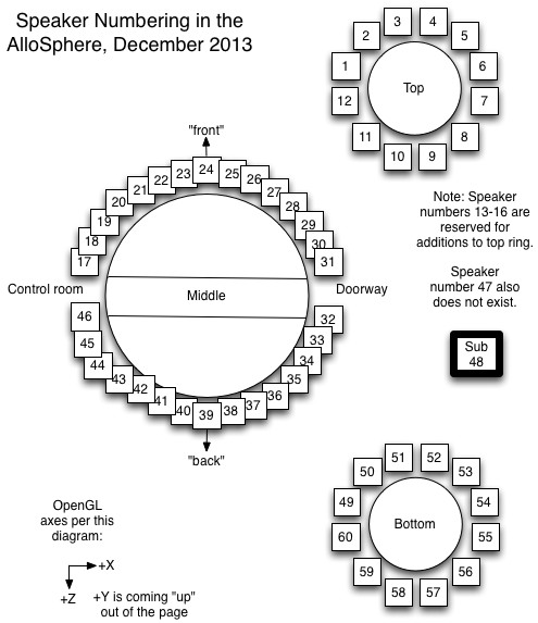
The speakers are arranged in 3 tiered circles: the bottom row and top rows have 12 speakers (each about 22% of the 54 speakers) and the middle row has the remaining 30 (about 56% of the speakers). I used a robust scaler to find the 22nd percentile and 78th percentile of mean spectral centroids in the dataset. I can then query the dataset to separate out sound slices for which the mean centroid is above the 78th percentile (and place them in the top circle of speakers), any sounds for which the mean centroid is below the 22nd percentile (and place them in the bottom row of speakers), and place all the sound slices in between in the middle row of speakers.

Once I had the slices separated out into these three groups (for the three speaker tiers), I used UMAP to reduce each group’s analyses of 13 mean MFCCs down to two dimensional space because each tier of speakers is on a 2D plane. Next, I used robust scaler to “center” the data to a median of zero so that the data would be centered around the origin [0,0]. I then computed the angle of each data point in relation to the “center” (using atan). This ignores the distance from the center, but this is ok because eventually I want all the points to be the same distance from the listener (the speakers are all the same radius distance), but evenly spread around the listener. After finding the angle of each data point, I sorted the points by angle and then spaced them evenly from 0 to two pi, quantized to the nearest speaker. I did this for each of the three tiers of speakers.

My initial plan was to map each slice to just one speaker and not have any speakers playing more than one slice at a time. In order to achieve this, I iterated over the slices in chronological order to place them in their assigned speaker. If a speaker was already playing back a slice (because there were many stems that might have overlapping slices), I tried moving the new slice to the opposite side of the circle of speakers. This might create a “stereo” effect using what seems to be two very similar slices (they might even be L and R from the original mix). This also is strategic for orchestration/mixing because if the two sound slices ended up on the same tier and in the same speaker they are probably similar spectra and therefore might cause masking if played from the same speaker. If the speaker on the opposite side also had a sound already playing, I chose a random available speaker for the sound slice in question.

Once I was in the room and heard the spatialization for the first time, the result was quite successful. I noticed that when musical gestures and phrases (comprised of a few slices) would repeat in the music, their spatial organization would repeat as well. These non-random, musically-determined correlations felt intentional and expressive even though they weren’t exactly determined by the composer. Because I only had a few hours in the space, it wouldn’t have been possible to intuitively compose these correlations in the room.

The speakers were rather small and not too loud so the actually presence of the sound was not as full as I had hoped. To remedy this, I end up spreading the sound of each speaker across it’s two adjacent speakers. This created a little more fullness and volume that was more pleasing to hear in the space. The musical-spatial organization created by the process described above was still clearly maintained even after this channel duplication.

Movement 2 & 4

For both of these movements I took the stems and decomposed them using NMF so that I could place different components in different speakers. For movement 2, I separately decomposed the left and right channels of the feedback sounds and the “eyeball” sounds into 20 components each (so a total of 40 components for feedback and 40 for eyeball). In movement 4, I did the same for 4 different stems containing the sinusoidal resynthesis sounds (although they’re not all playing at the same time).

I wanted to have the sounds be more spatially dynamic than just positioning each component in a different speaker, hopefully in a way that was aware of the content to some extent so that the sounds themselves could seem to be causing movement in space. I decided to move the signal to a random speaker each time an onset is detected (using SuperCollider’s Onsets.kr). Rather than using Ambisonics or VBAP, I chose a more efficient and more direct approach (something I’ve use in the Cube at Virginia Tech, which has 140+ speakers, so efficiency can be important), which is to essentially crossfade between two Out.ar buses that are being updated with the previous and current bus channels routed to the correct speakers. The channels can be spatially adjacent or not (if spatially adjacent, it resembles VBAP). For these moments in the Allosphere, I chose to not make them adjacent and just have the sounds dance around the room more randomly and freely.

In order to avoid unwanted artifacts when randomly changing the bus argument for Out.ar UGens I had to make sure to store what the previously used channel was (what speaker is being faded out) and the channel currently being crossfaded to (what speaker is being faded in). My solution was to use a LocalBuf of 2 frames as a “circle buffer”, to store the current and previous channels.

For Movement 3, nothing clever was done. I just took the stems and chose some speakers!

Video Design: Equirectangular Projection

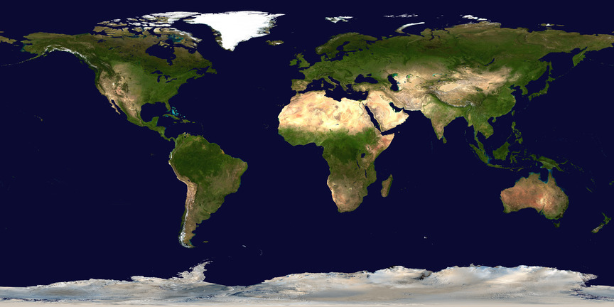
The video format that the Allosphere is able to display properly “on/in” the sphere is called equirectangular projection. It is a common projection for world maps (the one that makes Antarctica look like it spreads across the entire bottom of the map).

In the original work, the video design of movements 2, 3, and 4 are all very much oriented towards viewing it as a proscenium. Of course presenting it in the Allosphere would need some re-designing. The video design of the first movement is a little more flexible in that it is more chaotic, often expressing textures, shapes, lines, colors, etc. that are not necessarily tied to or intended for specific locations on the screen or in the viewer’s perception. This allows it to be mapped to the sphere a little more freely. Luckily, because equirectangular projection is a format often used for VR, Premiere Pro has a tool for controlling and previewing what it will look like from “inside” the sphere.

Movement 1

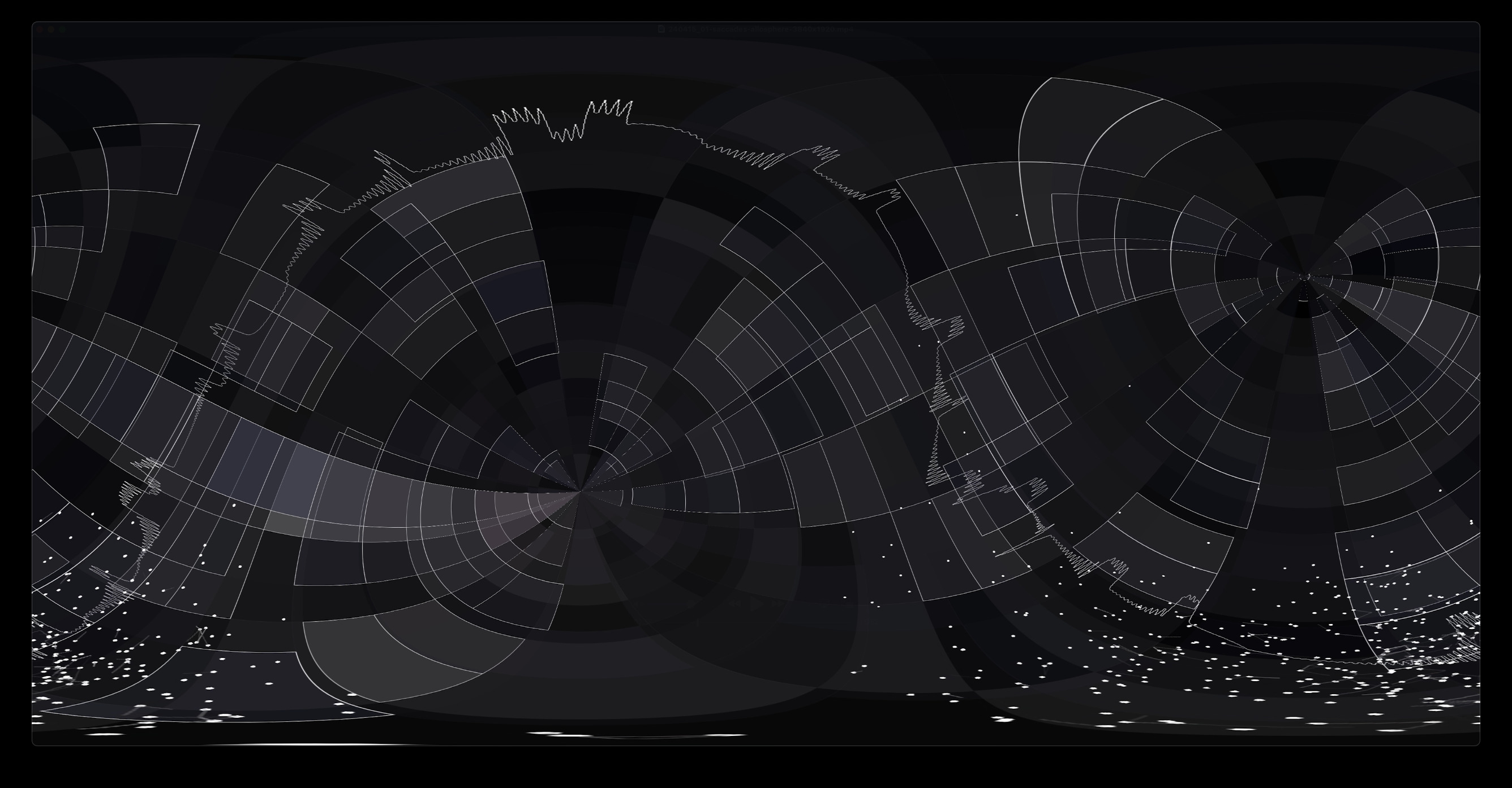
For the most part the 16:9 rectangle of the first movement is directly interpreted as “equirectangular” even though it is not. This means that the top and bottom edge are squished into one point at the north and south poles of the sphere and the areas around them are similarly distorted. This often created cascading arcs and circles of latitude and/or longitude on the sphere that were a pleasing result. One issue was that non-abstract moments, such as when the video was a full view of an eye, the image would absolutely not be perceptible in the sphere (because of the polar squishing, but also because it would be too large). For these moments I positioned the eye video smaller, somewhere in the sphere for the audience to view in a more “proscenium” format. I also often positioned more copies of the video in a geometric pattern to add interest. Another issue was the “seam” where the sides of the 16:9 video would meet on a longitudinal arc of the sphere. Since this is essentially unavoidable, I chose to “rotate” the projection so that this seam (and the polar points) would appear in different places at different times and move during some passages.

Movement 2

The original video design of movement two is comprised of a large view of the eyeball. Since this won’t work in the sphere (as described above) I placed the eyeball video in different “proscenium viewing” places each time it appeared. This alone seemed too simple so I decided to add a new element to the video design for this movement: each time the low pulse was heard, a new still image of an eyeball appeared (and another might disappear) somewhere in the sphere. Similar to the sound spatialization strategy from above, I wanted the positions of these images to not be random, but have some meaningful relationship to each other: I wanted similar looking images to be in similar spaces in the sphere. Since the viewing space is three dimensions ([x,y,z] or [angle,elevation,radius] but, yes, radius would be constant), I wanted to use a dimensionality reduction algorithm to embed the eyeball images into three dimensional space for determining their position in the sphere. The first step was to figure out how to represent these images as vectors that were meaningfully relevant to the content of the image (raw pixel values would not provide the comparisons and distinctions I was after). I used MediaPipe’s Image Embedder, which embeds any image into 1024 dimensional space. This embedding is often used for image comparison using cosine similarity, however I used it as the data set to embed these images down into the three dimensional space.

First I used PCA (since MediaPipe is in Python, I used sklearn for this ML pipeline) to reduce the number of dimensions from 1024 to the first 258 principal components which was able to maintain > 95% of the variance. I then used UMAP to reduce to 3 dimensions. I again used robust scaler to center the dimension’s medians to the origin for easier placement in the sphere.

This data would need to be positioned programmatically (as opposed to manually in a video editor), so I found the openFrameworks addon ofxEquiMap (which requires ofxCubeMap) to position images (in three dimensional space) in an equirectangular projection video which could be used in the Allosphere. This worked quite well. I was able to use the azimuth and elevation to position an image in space, and used the magnitude of the vector to position the image farther away, behind and smaller than images in front of it.

Movements 3 (and 4)

The blue lines were inspired by the blue line from the original video design of movement three and the blue bars of movement four. Because the original the blue video is a view of the ocean meeting the sky that slowly rotates 180 degrees, I chose to have these blue bands (showing a slice of the water video) rotate around the sphere. This was quite straightforward using Premiere Pro’s equirectangular projection rotation tools.

The fading in and out of the blue bars was done in the same way as the blue pillars in the fourth movement of the original video design: the tape part was decomposed (using NMF) into the the same number of components as there are bars and then the activations of the decomposition are used to modulate the alpha of the bars’ video. The result is not mickey-moused to the loudness, but still offers nice glimpses of audio-visual correlation.

The placement of the eyeball videos was done using the same openFrameworks code used in movement two. In order to simplify the code and not overload the computation, I rendered the equirectangular video one frame at a time (always fetching the next video frame for each of the eyeball videos and displaying it in the proper location). The positions of the video were chosen in two different ways (seen in different moments during the movement).

1. Video positions were selected randomly using a poisson-disc sampling strategy where a minimum arc distance between images on the surface of the sphere is tunable along with a maximum number of failed placements before determining that the space is “full” (both of these parameters are set using a .json config file supplied to the program at run time).
2. Video positions are fit together as closely as possible in a grid configuration. When positioned on the grid, each video could either start at a random frame, or, one frame later than the video that was positioned just before it. When adjacent videos’ start positions were offset by on frame, a pleasing “wave” effect appeared, where for example, the eye-closing gesture would be passed all around the rows of the sphere and move from the bottom to the top (watch for it in the excerpt).

In both cases the video was set to “palindrome” where it alternates playing a video forward and backward to avoid visual discontinuities. These different settings were rendered to equirectangular videos so that they could be further edited and combined in Premiere Pro.

Conclusion

Using these algorithmic/machine learning approaches to adapt saccades for the Allosphere not only sped up the process (I didn’t have much time leading up to the performance!) but also helped me “surf” the data in a way that didn’t require me to make specific decisions about all the facets of the huge “surface” of this space (three story video sphere and 54 speakers). Instead I could make specific decisions about how to organize sound in time and space creating large-scale, audio-visual-musical correlations to draw in the interest and curiosity of a viewer.